#Types of Machine Learning
In general, there are two types of machine learning: supervised and unsupervised. They’re pretty self-explanatory:
- Supervised learning looks at data with multiple inputs and their corresponding outputs, and produces a function that can take new input and produce accurate output.
- Unsupervised learning finds patterns in datasets without “correct” outputs. When humans have difficulty finding patterns in data, this can be beneficial.

#Neural Networks

A simplified visualization of what happens in a neural network. Source: Wikipedia. CC BY-SA 4.0
Artificial Neural Networks (ANN/NN), are a type of supervised machine learning model inspired from neurons in animal brains. In general, they:
- Read input data
- Determine output
- Compare determined output to the “correct” output
- Optimization
- Check if the model is done training. If not, repeat.
Each node in a neural network represents a neuron. Neurons exist in 3 types of layers:
- Input layer
- Intermediate layers known as hidden layers, which contain a vector known as a weight. If there are multiple hidden layers, the network is considered a deep neural network.
- Output layer
#Step 1: Input Data
Neural networks require a large amount of data in order to function efficiently. A single unit of input is called a sample, and is often expressed as a vector, e.g. [1.2, 3.4, 5.7, 2.9].
For the best result, separate the data into two parts: a training dataset (~80% of total data) for the model to train on, and a validation dataset (the remaining ~20%) to see how a trained model performs on unseen data.
#Step 2: Process Inputs and Determine Outputs
In order to calculate an output, the model has to send the inputs through each layer of the network, one by one. As the input is passed through each node, it goes through a complicated mathematical equation.
#Activation Functions
Just like how a real neuron either fires (represented by a 1) or doesn’t (0), a network’s activation function, represented as $\sigma(x)$, can simulate “firing” by normalizing output to a certain range like $(0,1)$ or $(-1,1)$. There are many common activation functions and each have their own advantages.
| Function Name | Definition |
|---|---|
| Step | $\sigma(x) = \begin{cases} x = 1, & x \geq 0 \\ x = 0, & x < 0\end{cases}$ |
| Linear | $\sigma(x)$ = x |
| Sigmoid | $\sigma(x) = \frac{1}{1-e^{-x}}$ |
| Tanh | $\sigma(x) = \frac{2}{1+e^{-2x}}$ |
| Rectified Linear Unit Function (ReLU) | $\sigma(x) = max(0, x)$ |
Common activation functions. Explanations here.
#Biases
Activation functions sometimes require weighted inputs to fall within a certain range in order to function effectively. If your weighted inputs don’t fall within this range, you shift the activation function’s effective range by adding a scalar $b$ called a bias.
Example: Sigmoid
Let’s say you decide to use the sigmoid activation function for one of your projects, and your inputs mostly contain values between -500 and -510. Since the sigmoid activation function (and lots of other activation functions) is basically 0 for any inputs less than -5, it is likely that no matter the weights, some layers may never output anything except for 0. To fix this, you could add 505 to your inputs whenever you process them. This way, the activation function is being applied to values within [-5, 5].
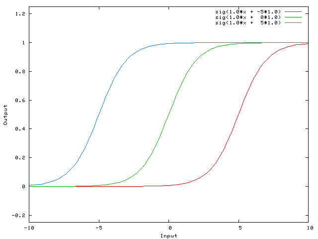
Sigmoid activation function with biases of -5 (blue), 0 (green), and 5 (red). Source: Stack Overflow, CC BY-SA 4.0
#Computations
In a network with $n$ layers, the network will process the input layer $l_1$ first, then hidden layers $l_2$, and so on through $l_{n-1}$, until reaching the output layer $l_n$. In this way, layers become dependent on previous layers.
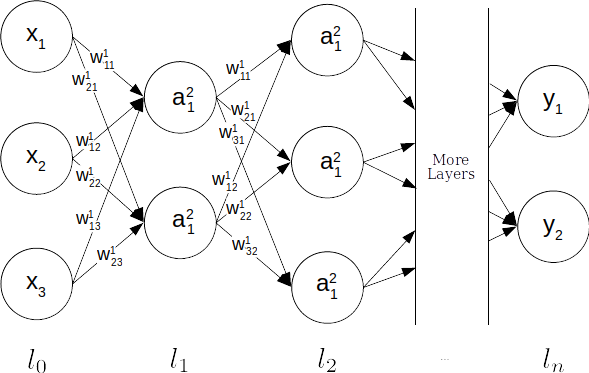
First, we determine our weighted input $z^l$, which is the current weight multiplied by the result of our last layer $a^{l-1}$ plus a bias $b$: $$ z^l = w^la^{l-1} + b^l $$
Finally, the output of neuron $a^l$ is defined as the activation function $\sigma(x)$ applied to the weighted input $z^l$.
$$ a^l = \sigma(z^l) = \sigma(w^la^{l-1} + b^l) $$
#Step 3: Comparison
Neural networks are a form of supervised learning, so once the neural network processes all inputs through the network, it compares the outputs it generated to what it should have generated.
This comparison requires a function that can calculate the difference. That special function is called a loss function.
#Loss Functions
The goal of the network is to reduce the difference between what we have and what we want; this difference is called the loss or cost, which is calculated using a loss function or cost function.
One common loss function is the mean squared error (MSE):
$$ MSE = \frac{1}{n}\sum_{i=1}^{n}(Y_{i}-\hat{Y_{i}})^{2} $$
#Step 4: Optimization
Optimization refers to the process a neural network goes through in order to improve. There are multiple Optimization Algorithms that each work a little differently, but the most common algorithm is known as Gradient Descent.
#Batch Size
Optimization takes a lot of time and processing, so it doesn’t always occur after every sample is processed: the batch size is the number of samples the model should work through before undergoing optimization.
| Batch Size (Samples) | Type of Optimization Algorithm |
|---|---|
| 1 | Stochastic Gradient Descent (SGD) |
| 1 < x < All | Mini-Batch Gradient Descent |
| All | Batch Gradient Descent |
Each algorithm has its pros and cons. In general, it is recommended to use mini-batch learning, because it is faster and more stable than stochastic learning and does not require all data to be present when training like batch learning.
#Step 5: Check: Are We Done Training?
A single epoch represents a cycle through all of the training data. It can take anywhere from <1 to 1000+ epochs to finish training, so how can we know when the model is sufficiently trained?
If the model is trained too little or too much, problems will arise:
#Undertraining
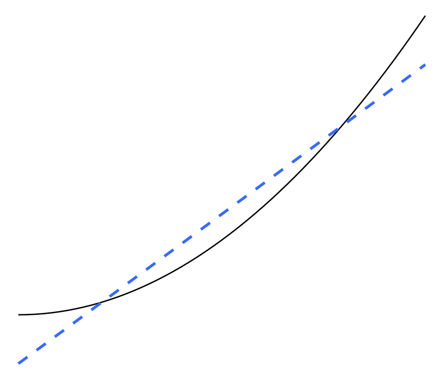
The training data lies along the blue parabola, and the dashed line represents an underfitted model. Although it may get some answers right, it has not captured the pattern (in this case, the curve). Source: Wikipedia, CC BY-SA 4.0
Undertraining results in underfitting, which is when the model cannot adequately capture the patterns that exist within the training data.
#Overtraining

The red and blue dots represent training data. The green line represents an overfitted model, clinging tightly to the training data. The black line represents a more sensible, regularized model. Source: Wikipedia, CC BY-SA 4.0
Overtraining results in overfitting. This means the model has produced a function that fits too closely to the training dataset; it has found patterns in the dataset that were not meant to be found. Think of this as the model “memorizing” the dataset rather than actually “learning” it.
#Example: Baby Names
For example, let’s say you want to train a model to produce English baby names, but most of your training data contains names that start with A. At first, the model might learn how to string together vowels and consonants to create syllables; next, it might learn that names do not contain punctuation.
Stopping training here would result in an underfitted model, because there are many more patterns that are yet to be learned. Eventually, it learns more common name patterns. However, if trained for too long, the model might start to find patterns it was never meant to. It may eventually think that because most of the baby names it sees start with an A, all baby names must start with an A. At this point, the model has overfit the training data.
#Early Stopping
In order to prevent undertraining or overtraining, we can use Early Stopping. The purpose of the validation set (~20% of your data) is to provide an unbiased evaluation of a machine learning model’s effectiveness. By periodically testing our model against this set, we can see whether or not it is overfitting the training data.

The blue line represents training set error, which is consistently decreasing. The red line represents validation set error, which decreases until the model begins overfitting, shown by the vertical line. Source: Wikimedia Commons, CC BY 3.0
As our model trains, it should perform better on the validation set. If error on the validation set increases for several consecutive optimizations, it is likely that overfitting as occurred, and training should stop.
#Conclusion
When effective training is completed, we are left with a neural network that is able to receive completely new input and use what it has learned to output sensible values. The applications of this type of machine are endless; we’ve only begun to see the power of machine learning. To see a cool showcase of AI, check out AI Dungeon.